Adverse Condition - Glaze

The goal of this section is to describe how we tackled the problem of improving lane detection performance in one of the adverse conditions - glaze. Lane detection can be challenging in the scenarios when there is glaze in the images which might obstruct a clear view of the environment outside. Glaze can occur because of the reflection of light off the windshield of the car. To tackle this, we propose a two step procedure. In the first step, we perform deglazing which is an attempt to recover as much information in the glaze region of the image based on the images dataset that we have. Once a deglazed image is retrieved, we train the SCNN model over this new dataset (deglazed images instead of glaze images + images from other scenarios) in the second step. The following sections describe these sections in more detail.

1. DeGlazing

Deglazing an image directly by itself is challenging because the glaze region in an image can be quite large as seen from sample images shown in Introduction section. This leads to a lot of information being lost in the corresponding regions. Therefore, we employed some heuristics to solve this problem. The first challenge was to identify the exact location of glaze in the image. To achieve this, we used an assumption that the glaze pixels are saturated. With this assumption, it is simple then to locate the glaze region by filtering the pixels in the image with the intensities above a threshold. We chose a threshold of 200. While doing this, it is also important to distinguish the glaze caused by reflection vs the bright sky outside which might also have some pixels above the threshold. To distinguish the glaze on windshield with the sun or sky, we only looked for glaze in the lower part of the image assuming that the saturated pixels in the top part of the image might be due to bright sky outside. We used three windows: left bottom, center bottom, and right bottom and selected the region with maximum number of saturated pixels as the region with glaze.

Once the region with glaze in an image is identified, the next and perhaps an even important step is to deglaze those pixels. Using just the training data that we had, we tried to interpolate the glaze pixels with corresponding pixels from the historical frames assuming that there might be some images in the recent past with less glaze at the corresponding pixel. We chose a window size of 5 historical frames. Initially, we tried simple interpolation, which we later modified with some advanced techniques such as incorporating the change in location of car from frame to frame. This technique of utilizing information from Optical Flow is described in more detailed later.

Optical Flow

After evaluating our results on deglazed images, we observed some drawbacks in heuristic per-pixel replacement approach. Firstly, it adds noise in the image, which is difficult to remove even with smoothing. This also makes it difficult to fit the spline curve which may further affect our results, even if our predictions may be correct. Second, it also may also lead to shift in predicted lane markings due to inherent motion present between neighbouring images. To overcome these, we tried the approach of using optical flow to incorporate the motion of car also while interpolating the pixels. We tried three different approaches for find the optical flow between the images as described below.

Methods:

1. Horn-Schunck Method:

Horn Schunck method assumes that the optical flow is smooth over the entire image and computes an estimate of the velocity field that minimizes the equation:

2. Lucas-Kanade Method:

Lucas-Kanade method assumes that the flow is essentially constant in a local neighborhood window $W$ of the pixel under consideration and solves the basic optical flow equations for all the pixels in the neighborhood by least squares criterion. That is, for all points $(k, l) \in W$, $I_x(k, l)u + I_y(k, l)v + I_t(k, l) = 0$

We used pre defined estimateFlow() method in MATLAB with opticalFlowHS for Horn-Shunck method and opticalFlowLK for Lucas-Kanade method for the opticFlow parameter.

3. Template-Matching Method:

In this method, for each template window $T$ in image $I_1$, first find the corresponding match in image $I_2$. Then the vector from the initial position to the final position of the corresponding points gives an estimate of optical flow at each point. We used Sum of Squared differences to compare the windows in image $I_1$ with the windows in image $I_2$.

We used the implementation from hw 7 for this.

Approach to interpolate glaze pixels with optical flow:

After trying the three methods described above, we found that the template-matching based approach worked best for the approach. Now, the goal is to incorporate the motion of the vehicle while interpolating the pixels with historical images in the glaze region. Optical flow can give us an estimate of how much the vehicle has moved compared to the previous frame and thus instead of interpolating the pixels based on just the corresponding coordinates in the image, we can add the optical flow vector to each pixel in the glaze region to get an estimate of the new position of the historical pixel point in the image.

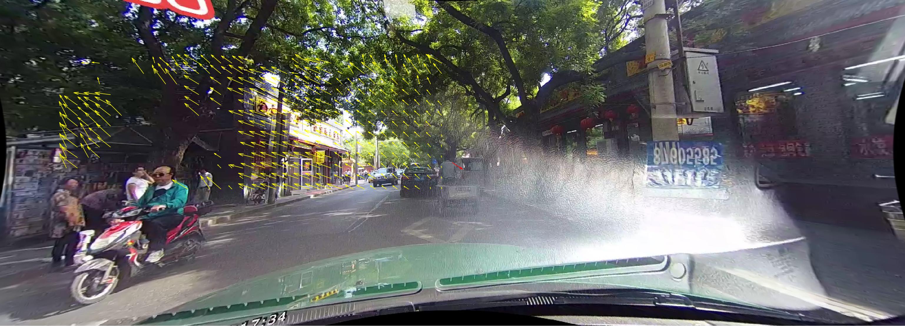
For this, we need to determine the optical flow direction and magnitude. But the challenge is that we cannot directly estimate the optical flow of the glaze region as these images are saturated which results in noisy optical flow. Therefore, we employ certain heuristics to do the same. Firstly, it is important to observe that due to the movement of the vehicle in forward direction, the dominant optical flow direction of the image in outward direction from the center of the image. We have also discarded the directions that do not agree with this dominant direction as those optical flow vectors can be considered noise. That is in the top left part of the image, the optical flow is in the left top direction, and in the bottom right part of the image, the optical flow is in the right bottom direction. Therefore, we take the opposite region of glaze in the image and estimate the optical flow direction to be the opposite of the average of the opposite region. The below images illustrate this:

As it can be seen from the figure, since the glaze region is in the right bottom, the optical flow was computed for the left top region. Only the vectors in the left top direction are kept and the others are discarded. These can be seen as a needle plot in yellow color. We then take the average of all these vectors and the opposite direction of this vector is assumed to be the optical flow of the glaze region. This is depicted by a small red colored vector in the center of the image. The same is repeated for getting the optical flow direction of the glaze region. Once we get this information, we incorporate the same to interpolate the glaze region pixels.

Since the region with the glaze pixels need not lie in a perfect region with good boundaries, we later realised that replacing at the level of pixels added some noise. To smoothen out this noise, we tried using Gaussian Smoothing in the glaze region but the results did not improve because of this.

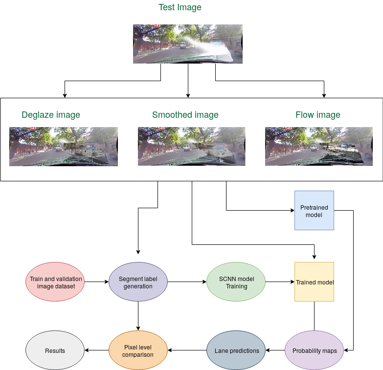
Once the images were deglazed, we used them for training a new model as described in SCNN Training section.. We also evaluated the results of these deglazed directly on pretrained model.

2. SCNN + DeGlaze Training

We trained the deglazed images created above using the tensorflow based implementation provided by SCNN-tensorflow. The model was trained on GPU machines provided by Wisconsin Applied Computing Center. The model for training takes as input the image files as well as their lane markings. The training requires per pixel labels, which are generated using a seperate method provided at Seg_label_generate.

Complete process flow

Segment label generation

This method tries to fit a spline curve by extrapolating the already present manual markings, and write out the per pixel labels. It also identifies the coordinates of the lanes using the provided manual points. The authors of SCNN use the same method for their training and evaluation.

The deglazed images were divided into validation, test and training sets contaning 100, 86, and 300 images respectively. We ran the training for 10000 iterations with intermittent checkpointing using a learning rate of 0.01 and nesterov momentum of 0.9. The GPU machines used were 4 Tesla V100-SXM2 with a memory fraction of 0.85. We trained the images in batch sizes of 8 using asynchronous training.

However, we observed that the number of images for training were very less and the model trained was not good. This calls for requirement of more data specific to glazing images to be able to perform training on them.

Testing SCNN + DeGlaze

We evaluate our results on both the pretrained model and our trained model created above. For testing on our model, we used a random subset of 100 images sampled above. The models predict probabilities for presence of lane at each pixel in the images. These probabilities map are then used to generate lane segment predictions. These lane predictions are then connected using spline curve fitting to form continous markings. The predicted lanes are compared with the labelled markings on a per-pixel basis, using the evaluation metric described below.